A near-infrared spectrum hands you two thousand highly correlated numbers to predict one — moisture, protein, octane. Ordinary regression drowns in that collinearity. Chemometrics survives it by refusing to work in wavelength space at all. Instead, everything happens in latent space: a handful of directions that carry the chemistry.
Why spectra demand latent variables
Adjacent wavelengths in a spectrum move together — that’s physics, not redundancy you can delete. With 2000 predictors and 80 samples, multiple linear regression is hopelessly underdetermined, and the predictors are nearly linear combinations of each other. Latent-variable methods solve both problems at once: project the spectra onto a few orthogonal directions, then regress on those.
PCA: the map of your data
Principal Component Analysis decomposes the spectral matrix into scores and loadings plus residual noise:
holds the sample coordinates in latent space, the wavelength directions, everything the model leaves behind. In practice:
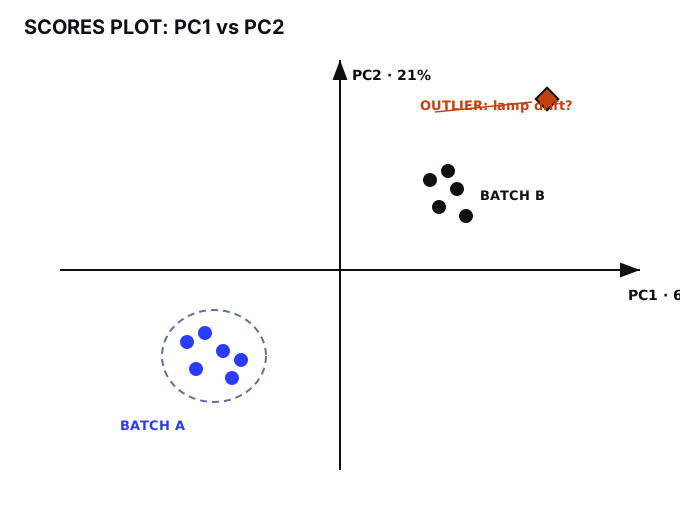
- Scores are your samples in latent space. Plot PC1 vs PC2 first, always — clusters reveal batches, outliers scream, and drift across measurement days shows up as a slow march across the plot. Half of chemometrics troubleshooting is staring at score plots.
PLS: latent space with a purpose
Partial Least Squares builds latent variables that maximize covariance with your target, not just variance in the spectra. Both blocks share the same scores:
Same machinery, pointed at the problem. Two disciplines separate good PLS from numerology:
- Component count is the whole ballgame. Each added latent variable fits a little more signal and a little more noise. Select it by cross-validation (venetian blinds or contiguous blocks for batch data — never leave-one-out on spectra, it’s optimistically biased), and prefer the simplest model within noise of the minimum error.
- Validate like the instrument will be used. Random splits of spectra from the same batch leak; the model memorizes the batch, not the chemistry. Hold out entire batches, days, or instruments. If performance collapses, your latent space encoded the lab, not the analyte.
Reading the latent space
A trained model’s loadings are a hypothesis about chemistry. Check them: do the PLS weights peak at wavelengths your domain knowledge expects? If the “moisture model” loads heavily on a region with no water absorption, it’s riding a confounder — temperature drift, particle size, a lamp change. The model will work until the confounder shifts, then fail silently. Interpretability isn’t a luxury in chemometrics; it’s the only early-warning system you have.
Preprocessing is part of the latent space too. SNV, MSC, derivatives — these aren’t rituals, they’re choices about which variation gets to enter the projection. Scatter correction removes physical variation (particle size) so the latent variables can spend their capacity on chemistry. Get preprocessing wrong and your first three components model the sample grinder.
Autoencoders: the nonlinear temptation
A bottleneck autoencoder learns a nonlinear latent space that can capture curved structure PCA misses. Tempting — but you trade the loading plot for a black box, and with 80 spectra and 2000 wavelengths, a deep network will memorize with enthusiasm. If you go there: heavy regularization, tiny bottlenecks, and the same batch-aware validation. Usually, well-preprocessed PLS with the right component count wins on small spectral datasets, and you can still read its mind afterward.
The checklist
- Score plots before models — know your batches, outliers, and drift
- PLS components by honest cross-validation; simplest within noise wins
- Hold out whole batches/days/instruments, never random spectra
- Read the loadings: chemistry or confounder?
- Preprocess deliberately — decide what variation deserves latent capacity
Spectra are high-dimensional, but chemistry is low-dimensional. Latent space is just the discipline of finding out how low.
← All posts